Introduction
Package nuggets searches for patterns that can be
expressed as formulae in the form of elementary conjunctions, referred
to in this text as conditions. Conditions are constructed from
predicates, which correspond to data columns. The
interpretation of conditions depends on the choice of underlying
logic:
Crisp (Boolean) logic: each predicate takes values
TRUE(1) orFALSE(0). The truth value of a condition is computed according to the rules of classical Boolean algebra.-
Fuzzy logic: each predicate is assigned a truth degree from the interval \([0, 1]\). The truth degree of a conjunction is then computed using a chosen triangular norm (t-norm). The package supports three common t-norms, which are defined for predicates’ truth degrees \(a, b \in [0, 1]\) as follows:
- Gödel (minimum) t-norm: \(\min(a, b)\) ;
- Goguen (product) t-norm: \(a \cdot b\) ;
- Łukasiewicz t-norm: \(\max(0, a + b - 1)\)
Before applying nuggets, data columns intended as
predicates must be prepared either by dichotomization
(conversion into dummy logical variables) or by transformation
into fuzzy sets. The package provides functions for both
transformations. See the section Data
Preparation below for a quick overview, or the Data Preparation vignette for a
comprehensive guide.
nuggets implements functions to search for pre-defined
types of patterns or to discover patterns of user-defined type.
For example, the package provides:
-
dig_associations()for association rules, -
dig_baseline_contrasts(),dig_complement_contrasts(), anddig_paired_baseline_contrasts()for various contrast patterns on numeric variables, -
dig_correlations()for conditional correlations.
To provide custom evaluation functions for conditions and to search for user-defined types of patterns, the package offers two general functions:
-
dig()is a general function for searching arbitrary pattern types. -
dig_grid()is a wrapper arounddig()for patterns defined by conditions and a pair of columns evaluated by a user-defined function.
See the section Pre-defined Patterns below for examples and details on using the pre-defined pattern discovery functions and the section Advanced Use for examples of custom pattern discovery.
Discovered rules and patterns can be post-processed, visualized, and explored interactively. That part is covered in the section Post-processing and Visualization below.
Data Preparation
Before applying nuggets, data columns intended as
predicates must be prepared either by dichotomization
(conversion into dummy variables) or by transformation into
fuzzy sets. The package provides the partition()
function for both transformations.
This section gives a quick overview of data preparation with
nuggets. For a detailed guide, including information about
all available functions and advanced techniques, please see the Data Preparation Vignette.
Crisp (Boolean) Predicates Example
For crisp patterns, numeric columns are transformed to logical
(TRUE/FALSE) columns. To show the process, we
start with the built-in mtcars dataset, which we first
slightly modify by converting the cyl column to a
factor:
# For demonstration, convert 'cyl' column of the mtcars dataset to a factor
mtcars <- mtcars |>
    mutate(cyl = factor(cyl, levels = c(4, 6, 8), labels = c("four", "six", "eight")))

head(mtcars, n = 3)
#>                mpg  cyl disp  hp drat    wt  qsec vs am gear carb
#> Mazda RX4     21.0  six  160 110 3.90 2.620 16.46  0  1    4    4
#> Mazda RX4 Wag 21.0  six  160 110 3.90 2.875 17.02  0  1    4    4
#> Datsun 710    22.8 four  108  93 3.85 2.320 18.61  1  1    4    1
Now we can use the partition() function to transform all
columns into crisp predicates:
# Transform the whole dataset to crisp predicates
crisp_mtcars <- mtcars |>
    partition(cyl, vs:gear, .method = "dummy") |>
    partition(mpg, .method = "crisp", .breaks = c(-Inf, 15, 20, 30, Inf)) |>
    partition(disp:carb, .method = "crisp", .breaks = 3)

head(crisp_mtcars, n = 3)
#> # A tibble: 3 × 32
#>   `cyl=four` `cyl=six` `cyl=eight` `vs=0` `vs=1` `am=0` `am=1` `gear=3` `gear=4`
#>   <lgl>      <lgl>     <lgl>       <lgl>  <lgl>  <lgl>  <lgl>  <lgl>    <lgl>
#> 1 FALSE      TRUE      FALSE       TRUE   FALSE  FALSE  TRUE   FALSE    TRUE
#> 2 FALSE      TRUE      FALSE       TRUE   FALSE  FALSE  TRUE   FALSE    TRUE
#> 3 TRUE       FALSE     FALSE       FALSE  TRUE   FALSE  TRUE   FALSE    TRUE
#>   `gear=5` `mpg=(-Inf;15]` `mpg=(15;20]` `mpg=(20;30]` `mpg=(30;Inf]`
#>   <lgl>    <lgl>           <lgl>         <lgl>         <lgl>
#> 1 FALSE    FALSE           FALSE         TRUE          FALSE
#> 2 FALSE    FALSE           FALSE         TRUE          FALSE
#> 3 FALSE    FALSE           FALSE         TRUE          FALSE
#>   `disp=(-Inf;205]` `disp=(205;338]` `disp=(338;Inf]` `hp=(-Inf;146]`
#>   <lgl>             <lgl>            <lgl>            <lgl>
#> 1 TRUE              FALSE            FALSE            TRUE
#> 2 TRUE              FALSE            FALSE            TRUE
#> 3 TRUE              FALSE            FALSE            TRUE
#>   `hp=(146;241]` `hp=(241;Inf]` `drat=(-Inf;3.48]` `drat=(3.48;4.21]`
#>   <lgl>          <lgl>          <lgl>              <lgl>
#> 1 FALSE          FALSE          FALSE              TRUE
#> 2 FALSE          FALSE          FALSE              TRUE
#> 3 FALSE          FALSE          FALSE              TRUE
#>   `drat=(4.21;Inf]` `wt=(-Inf;2.82]` `wt=(2.82;4.12]` `wt=(4.12;Inf]`
#>   <lgl>             <lgl>            <lgl>            <lgl>
#> 1 FALSE             TRUE             FALSE            FALSE
#> 2 FALSE             FALSE            TRUE             FALSE
#> 3 FALSE             TRUE             FALSE            FALSE
#>   `qsec=(-Inf;17.3]` `qsec=(17.3;20.1]` `qsec=(20.1;Inf]` `carb=(-Inf;3.33]`
#>   <lgl>              <lgl>              <lgl>             <lgl>
#> 1 TRUE               FALSE              FALSE             FALSE
#> 2 TRUE               FALSE              FALSE             FALSE
#> 3 FALSE              TRUE               FALSE             TRUE
#>   `carb=(3.33;5.67]` `carb=(5.67;Inf]`
#>   <lgl>              <lgl>
#> 1 TRUE               FALSE
#> 2 TRUE               FALSE
#> 3 FALSE              FALSE
As seen above, the "dummy" method can be used to create
logical columns for each category of processed variables. Here, it was
applied to create dummy variables for the factor variable
cyl as well as for the numeric variables vs,
am, and gear.
The method "crisp" creates logical columns representing
intervals for numeric variables. In the example, it was used to create
intervals for mpg based on specified breakpoints
(-Inf, 15, 20, 30,
Inf), and for disp, hp,
drat, wt, qsec, and
carb using equal-width intervals (3 intervals each).
Now all columns are logical and can be used as predicates in crisp conditions.
Fuzzy Predicates Example
Fuzzy predicates express the degree to which a condition is satisfied, with values in the interval \([0,1]\). This allows modeling of smooth transitions between categories:
# Start with fresh mtcars and transform to fuzzy predicates
fuzzy_mtcars <- mtcars |>
    partition(cyl, vs:gear, .method = "dummy") |>
    partition(mpg, .method = "triangle", .breaks = c(-Inf, 15, 20, 30, Inf)) |>
    partition(disp:carb, .method = "triangle", .breaks = 3)

head(fuzzy_mtcars, n = 3)
#> # A tibble: 3 × 31
#>   `cyl=four` `cyl=six` `cyl=eight` `vs=0` `vs=1` `am=0` `am=1` `gear=3` `gear=4`
#>   <lgl>      <lgl>     <lgl>       <lgl>  <lgl>  <lgl>  <lgl>  <lgl>    <lgl>
#> 1 FALSE      TRUE      FALSE       TRUE   FALSE  FALSE  TRUE   FALSE    TRUE
#> 2 FALSE      TRUE      FALSE       TRUE   FALSE  FALSE  TRUE   FALSE    TRUE
#> 3 TRUE       FALSE     FALSE       FALSE  TRUE   FALSE  TRUE   FALSE    TRUE
#>   `gear=5` `mpg=(-Inf;15;20)` `mpg=(15;20;30)` `mpg=(20;30;Inf)`
#>   <lgl>                 <dbl>            <dbl>             <dbl>
#> 1 FALSE                     0             0.9               0.1
#> 2 FALSE                     0             0.9               0.1
#> 3 FALSE                     0             0.72              0.28
#>   `disp=(-Inf;71.1;272)` `disp=(71.1;272;472)` `disp=(272;472;Inf)`
#>                    <dbl>                 <dbl>                <dbl>
#> 1                  0.557                 0.443                    0
#> 2                  0.557                 0.443                    0
#> 3                  0.816                 0.184                    0
#>   `hp=(-Inf;52;194)` `hp=(52;194;335)` `hp=(194;335;Inf)`
#>                <dbl>             <dbl>              <dbl>
#> 1              0.592             0.408                  0
#> 2              0.592             0.408                  0
#> 3              0.711             0.289                  0
#>   `drat=(-Inf;2.76;3.84)` `drat=(2.76;3.84;4.93)` `drat=(3.84;4.93;Inf)`
#>                     <dbl>                   <dbl>                  <dbl>
#> 1                       0                   0.945                0.0550
#> 2                       0                   0.945                0.0550
#> 3                       0                   0.991                0.00917
#>   `wt=(-Inf;1.51;3.47)` `wt=(1.51;3.47;5.42)` `wt=(3.47;5.42;Inf)`
#>                   <dbl>                 <dbl>                <dbl>
#> 1                 0.434                 0.566                    0
#> 2                 0.304                 0.696                    0
#> 3                 0.587                 0.413                    0
#>   `qsec=(-Inf;14.5;18.7)` `qsec=(14.5;18.7;22.9)` `qsec=(18.7;22.9;Inf)`
#>                     <dbl>                   <dbl>                  <dbl>
#> 1                  0.533                    0.467                      0
#> 2                  0.4                      0.6                        0
#> 3                  0.0214                   0.979                      0
#>   `carb=(-Inf;1;4.5)` `carb=(1;4.5;8)` `carb=(4.5;8;Inf)`
#>                 <dbl>            <dbl>              <dbl>
#> 1               0.143            0.857                  0
#> 2               0.143            0.857                  0
#> 3               1                0                      0
Similar to the crisp example, the "dummy" method creates
logical columns for categorical variables (cyl,
vs, am, gear).
The "triangle" method creates fuzzy predicates with
triangular membership functions. For mpg, it uses specified
breakpoints to define fuzzy intervals. For the remaining numeric
variables (disp through carb), it
automatically creates 3 overlapping fuzzy sets with smooth transitions
between intervals.
Note that the cyl, vs, am, and
gear columns are still represented by dummy logical
columns, while the numeric columns are now represented by fuzzy sets.
This combination allows both crisp and fuzzy predicates to be used
together in pattern discovery.
Advanced Data Preparation Capabilities
The nuggets package provides powerful and flexible data
preparation tools. The Data
Preparation vignette covers these capabilities in depth,
including:
-
Crisp (Boolean) partitioning with customizable
interval strategies:
- Equal-width intervals for uniform discretization
- Data-driven methods (quantile, k-means, hierarchical clustering, etc.) for optimal breakpoints that respect the data structure
- Custom breakpoints for domain-specific intervals
-
Fuzzy partitioning for modeling gradual transitions
and uncertainty:
- Triangular membership functions for basic fuzzy sets
- Raised-cosine membership functions for smoother transitions
- Trapezoidal shapes using
.spanand.incparameters for overlapping fuzzy sets
-
Quality control utilities to improve pattern
mining:
-
is_almost_constant()andremove_almost_constant()to identify and filter uninformative columns -
dig_tautologies()to find always-true or almost-always-true rules that can be used to prune search spaces
-
- Custom labels for predicates to make discovered patterns more interpretable
For example, you can use quantile-based partitioning to ensure balanced predicates, or use raised-cosine fuzzy sets with custom labels to create meaningful linguistic terms like “very_low”, “low”, “medium”, “high”, and “very_high”. These preparation choices significantly impact the interpretability and usefulness of patterns discovered in subsequent analyses.
Pre-defined Patterns
The package nuggets provides a set of functions for
discovering some of the best-known pattern types. These functions can
process Boolean data, fuzzy data, or both. Each function returns a
tibble, where every row represents one detected pattern.
Note: This section assumes that the data have already been preprocessed — i.e., transformed into a binarized or fuzzified form. See the previous section Data Preparation for details on how to prepare your dataset (for example,
crisp_mtcarsandfuzzy_mtcars).
For more advanced workflows — such as defining custom pattern types or computing user-defined measures — see the section Advanced Use.
Search for Association Rules
Association rules identify conditions (antecedents) under which a specific feature (consequent) is present very often.
\[ A \Rightarrow C \]
If condition A is satisfied, then the feature
C tends to be present.
For example,
university_edu & middle_age & IT_industry => high_income
can be read as:
In practice, the antecedent A is a set of predicates,
and the consequent C is usually a single predicate.
For a set of predicates \(I\), let \(\text{supp}(I)\) denote the support — the relative frequency (for logical data) or the mean truth degree (for fuzzy data) of rows satisfying all predicates in \(I\). Using this notation, the following rule properties and quality measures may be defined:
-
Length — number of predicates in the
antecedent.
-
Coverage (antecedent support) — \(\text{supp}(A)\).
-
Consequent support — \(\text{supp}(C)\).
-
Support — \(\text{supp}(A
\cup C)\).
- Confidence — \(\text{supp}(A \cup C) / \text{supp}(A)\).
- Lift — \(\text{supp}(A \cup C) / (\text{supp}(A) \text{supp}(C))\).
Rules with high support are frequent in the data. Rules with high confidence indicate a strong association between antecedent and consequent. Rules with high lift suggest that the validity of antecedent increases the likelihood of the consequent occurring.
Before searching for rules, it is recommended to create a vector of disjoints, which specifies predicates that must not appear together in the same condition. This vector should have the same length as the number of dataset columns.
For example, columns representing gear=3 and
gear=4 are mutually exclusive, so their shared group label
in disj prevents meaningless conditions like
gear=3 & gear=4. You can conveniently generate this
vector with var_names():
disj <- var_names(colnames(fuzzy_mtcars))
print(disj)
#>  [1] "cyl"  "cyl"  "cyl"  "vs"   "vs"   "am"   "am"   "gear" "gear" "gear"
#> [11] "mpg"  "mpg"  "mpg"  "disp" "disp" "disp" "hp"   "hp"   "hp"   "drat"
#> [21] "drat" "drat" "wt"   "wt"   "wt"   "qsec" "qsec" "qsec" "carb" "carb"
#> [31] "carb"
The dig_associations() function searches for association
rules. Its main arguments are:
-
x: the data matrix or data frame (logical or numeric); -
antecedent,consequent: tidyselect expressions selecting columns for each side of the rule; -
disjoint: a vector defining mutually exclusive predicates; - rule filtering thresholds such as
min_support,min_confidence,min_coverage, and limits likemin_length,max_length; - optional parameters such as
t_norm.
In the following example, we search for fuzzy association rules in
the dataset fuzzy_mtcars, such that:
- any column except those starting with
"am"may appear in the antecedent; - columns starting with
"am"may appear in the consequent; - minimum support is
0.02, i.e., 2 % of data rows have to contain both the antecedent and consequent of the rule; - minimum confidence is
0.8, i.e., the conditional probability of consequent given antecedent should be at least 80%.
result <- dig_associations(fuzzy_mtcars,
                           antecedent = !starts_with("am"),
                           consequent = starts_with("am"),
                           disjoint = disj,
                           min_support = 0.02,
                           min_confidence = 0.8)
The result is a tibble containing the discovered rules. Additional quality metrics may be computed:
result <- add_interest(result, measures = c("conviction", "leverage"))You can arrange the resulting rules, for example, by decreasing support:
result <- arrange(result, desc(support))
print(result)
#> # A tibble: 526 × 15
#>    antecedent                     consequent support confidence coverage
#>    <chr>                          <chr>        <dbl>      <dbl>    <dbl>
#>  1 {gear=3}                       {am=0}       0.469      1        0.469
#>  2 {gear=3,vs=0}                  {am=0}       0.375      1        0.375
#>  3 {cyl=eight,gear=3,vs=0}        {am=0}       0.375      1        0.375
#>  4 {cyl=eight,vs=0}               {am=0}       0.375      0.857    0.438
#>  5 {cyl=eight,gear=3}             {am=0}       0.375      1        0.375
#>  6 {cyl=eight}                    {am=0}       0.375      0.857    0.438
#>  7 {mpg=(-Inf;15;20)}             {am=0}       0.327      0.847    0.387
#>  8 {drat=(-Inf;2.76;3.84)}        {am=0}       0.311      0.948    0.328
#>  9 {gear=3,mpg=(-Inf;15;20)}      {am=0}       0.309      1        0.309
#> 10 {drat=(-Inf;2.76;3.84),gear=3} {am=0}       0.307      1        0.307
#>    conseq_support  lift count antecedent_length    pp    pn    np    nn
#>             <dbl> <dbl> <dbl>             <int> <dbl> <dbl> <dbl> <dbl>
#>  1          0.594  1.68 15                    1 15    0      4     13
#>  2          0.594  1.68 12                    2 12    0      7     13
#>  3          0.594  1.68 12                    3 12    0      7     13
#>  4          0.594  1.44 12                    2 12    2      7     11
#>  5          0.594  1.68 12                    2 12    0      7     13
#>  6          0.594  1.44 12                    1 12    2      7     11
#>  7          0.594  1.43 10.5                  1 10.5  1.90   8.52  11.1
#>  8          0.594  1.60  9.96                 1  9.96 0.546  9.04  12.5
#>  9          0.594  1.68  9.88                 2  9.88 0      9.12  13
#> 10          0.594  1.68  9.82                 2  9.82 0      9.18  13
#>    conviction leverage
#>         <dbl>    <dbl>
#>  1     Inf      0.190
#>  2     Inf      0.152
#>  3     Inf      0.152
#>  4       2.84   0.115
#>  5     Inf      0.152
#>  6       2.84   0.115
#>  7       2.65   0.0978
#>  8       7.82   0.116
#>  9     Inf      0.125
#> 10     Inf      0.125
#> # ℹ 516 more rows
This example illustrates the typical workflow for mining association
rules with nuggets. The same structure and arguments apply
when analyzing either fuzzy or Boolean datasets.
Conditional Correlations
Conditional correlations identify strong relationships between pairs of numeric variables under specific conditions.
The dig_correlations() function searches for pairs of
variables that are significantly correlated within sub-data satisfying
generated conditions. This is useful for discovering context-dependent
relationships.
In the following example, we search for correlations between
different numeric variables in the original mtcars data
under conditions defined by the prepared predicates in
crisp_mtcars:
# Prepare combined dataset with both condition predicates and numeric variables
combined_mtcars <- cbind(crisp_mtcars, mtcars[, c("mpg", "disp", "hp", "wt")])

# Extend disjoint vector for the new numeric columns
disj_combined <- c(var_names(colnames(crisp_mtcars)),
                   c("mpg", "disp", "hp", "wt"))

# Search for conditional correlations
corr_result <- dig_correlations(combined_mtcars,
                                condition = colnames(crisp_mtcars),
                                xvars = c("mpg", "hp"),
                                yvars = c("wt", "disp"),
                                disjoint = disj_combined,
                                min_length = 1,
                                max_length = 2,
                                min_support = 0.2,
                                method = "pearson")

print(corr_result)
#> # A tibble: 536 × 10
#>    condition               support xvar  yvar  estimate     p_value
#>    <chr>                     <dbl> <chr> <chr>    <dbl>       <dbl>
#>  1 {carb=(-Inf;3.33]}        0.625 mpg   wt      -0.887 0.000000183
#>  2 {carb=(-Inf;3.33]}        0.625 mpg   disp    -0.816 0.0000116
#>  3 {carb=(-Inf;3.33]}        0.625 hp    wt       0.791 0.0000326
#>  4 {carb=(-Inf;3.33]}        0.625 hp    disp     0.877 0.000000388
#>  5 {am=0,carb=(-Inf;3.33]}   0.375 mpg   wt      -0.632 0.0274
#>  6 {am=0,carb=(-Inf;3.33]}   0.375 mpg   disp    -0.633 0.0270
#>  7 {am=0,carb=(-Inf;3.33]}   0.375 hp    wt       0.755 0.00453
#>  8 {am=0,carb=(-Inf;3.33]}   0.375 hp    disp     0.813 0.00131
#>  9 {carb=(-Inf;3.33],vs=0}   0.25  mpg   wt      -0.823 0.0121
#> 10 {carb=(-Inf;3.33],vs=0}   0.25  mpg   disp    -0.585 0.128
#>    method                               alternative     n condition_length
#>    <chr>                                <chr>       <int>            <int>
#>  1 Pearson's product-moment correlation two.sided      20                1
#>  2 Pearson's product-moment correlation two.sided      20                1
#>  3 Pearson's product-moment correlation two.sided      20                1
#>  4 Pearson's product-moment correlation two.sided      20                1
#>  5 Pearson's product-moment correlation two.sided      12                2
#>  6 Pearson's product-moment correlation two.sided      12                2
#>  7 Pearson's product-moment correlation two.sided      12                2
#>  8 Pearson's product-moment correlation two.sided      12                2
#>  9 Pearson's product-moment correlation two.sided       8                2
#> 10 Pearson's product-moment correlation two.sided       8                2
#> # ℹ 526 more rows
This example combines crisp predicates (from
crisp_mtcars) with numeric variables from the original
mtcars dataset. The function searches for conditions under
which pairs of numeric variables show significant Pearson correlations.
The disjoint vector is extended to include the new numeric
columns, preventing conflicts in the search algorithm.
The result shows conditions under which specific pairs of variables exhibit strong correlations, along with correlation coefficients and p-values.
Contrast Patterns
Contrast patterns identify conditions under which numeric variables
show statistically significant differences. The nuggets
package provides several functions for different types of contrasts.
Baseline Contrasts
Baseline contrasts identify conditions under which a variable is significantly different from a baseline value (typically zero) using a one-sample statistical test.
# Prepare combined dataset with predicates and numeric variables
combined_mtcars2 <- cbind(crisp_mtcars,
                          mtcars[, c("mpg", "hp", "wt")])

# Extend disjoint vector for the new numeric columns
disj_combined2 <- c(var_names(colnames(crisp_mtcars)),
                    c("mpg", "hp", "wt"))

# Search for baseline contrasts
baseline_result <- dig_baseline_contrasts(combined_mtcars2,
                                         condition = colnames(crisp_mtcars),
                                         vars = c("mpg", "hp", "wt"),
                                         disjoint = disj_combined2,
                                         min_length = 1,
                                         max_length = 2,
                                         min_support = 0.2,
                                         method = "t")

head(baseline_result)
#> # A tibble: 6 × 15
#>   condition               support var   estimate statistic    df  p_value     n
#>   <chr>                     <dbl> <chr>    <dbl>     <dbl> <dbl>    <dbl> <int>
#> 1 {carb=(-Inf;3.33]}        0.625 mpg      22.5       17.1    19 5.45e-13    20
#> 2 {carb=(-Inf;3.33]}        0.625 hp      116.        11.5    19 5.16e-10    20
#> 3 {carb=(-Inf;3.33]}        0.625 wt        2.88      15.9    19 1.97e-12    20
#> 4 {am=0,carb=(-Inf;3.33]}   0.375 mpg      18.8       20.9    11 3.33e-10    12
#> 5 {am=0,carb=(-Inf;3.33]}   0.375 hp      138.        11.4    11 2.01e- 7    12
#> 6 {am=0,carb=(-Inf;3.33]}   0.375 wt        3.44      28.6    11 1.13e-11    12
#>   conf_lo conf_hi stderr alternative method            comment condition_length
#>     <dbl>   <dbl>  <dbl> <chr>       <chr>             <chr>              <int>
#> 1   19.8    25.3   1.32  two.sided   One Sample t-test ""                     1
#> 2   94.7   137.   10.0   two.sided   One Sample t-test ""                     1
#> 3    2.50    3.26  0.181 two.sided   One Sample t-test ""                     1
#> 4   16.8    20.8   0.900 two.sided   One Sample t-test ""                     2
#> 5  112.    165.   12.2   two.sided   One Sample t-test ""                     2
#> 6    3.18    3.71  0.120 two.sided   One Sample t-test ""                     2
This example tests whether the mean of numeric variables
(mpg, hp, wt) significantly
differs from zero under various conditions. The
method = "t" parameter specifies a t-test. The results show
which combinations of conditions lead to statistically significant
deviations from the baseline.
Complement Contrasts
Complement contrasts identify conditions under which a variable differs significantly between elements that satisfy the condition and those that don’t.
complement_result <- dig_complement_contrasts(combined_mtcars2,
                                             condition = colnames(crisp_mtcars),
                                             vars = c("mpg", "hp", "wt"),
                                             disjoint = disj_combined2,
                                             min_length = 1,
                                             max_length = 2,
                                             min_support = 0.15,
                                             method = "t")

head(complement_result)
#> # A tibble: 6 × 17
#>   condition                        support var   estimate_x estimate_y statistic
#>   <chr>                              <dbl> <chr>      <dbl>      <dbl>     <dbl>
#> 1 {carb=(-Inf;3.33]}                 0.625 mpg        22.5       16.0       3.80
#> 2 {carb=(-Inf;3.33]}                 0.625 hp        116.       198.       -3.60
#> 3 {carb=(-Inf;3.33]}                 0.625 wt          2.88       3.78     -2.61
#> 4 {carb=(-Inf;3.33],hp=(-Inf;146]}   0.406 mpg        25.6       16.3       6.04
#> 5 {carb=(-Inf;3.33],hp=(-Inf;146]}   0.406 hp         86.5      188.       -6.95
#> 6 {carb=(-Inf;3.33],hp=(-Inf;146]}   0.406 wt          2.45       3.74     -5.02
#>      df     p_value   n_x   n_y conf_lo conf_hi stderr alternative
#>   <dbl>       <dbl> <int> <int>   <dbl>   <dbl>  <dbl> <chr>
#> 1  29.9 0.000662       20    12    2.99   9.94   1.70  two.sided
#> 2  16.3 0.00233        20    12 -131.   -34.1   22.9   two.sided
#> 3  19.5 0.0171         20    12   -1.61  -0.178  0.343 two.sided
#> 4  18.5 0.00000929     13    19    6.06  12.5    1.54  two.sided
#> 5  24.3 0.000000318    13    19 -132.   -71.3   14.6   two.sided
#> 6  28.9 0.0000244      13    19   -1.82  -0.768  0.258 two.sided
#>   method                  comment condition_length
#>   <chr>                   <chr>              <int>
#> 1 Welch Two Sample t-test ""                     1
#> 2 Welch Two Sample t-test ""                     1
#> 3 Welch Two Sample t-test ""                     1
#> 4 Welch Two Sample t-test ""                     2
#> 5 Welch Two Sample t-test ""                     2
#> 6 Welch Two Sample t-test ""                     2
This example uses a two-sample t-test to compare the mean values of numeric variables between rows that satisfy a condition and rows that don’t. The results identify conditions where subgroups have significantly different characteristics compared to the rest of the data.
Paired Baseline Contrasts
Paired baseline contrasts identify conditions under which there is a significant difference between two paired numeric variables.
paired_result <- dig_paired_baseline_contrasts(combined_mtcars2,
                                              condition = colnames(crisp_mtcars),
                                              xvars = c("mpg", "hp"),
                                              yvars = c("wt", "wt"),
                                              disjoint = disj_combined2,
                                              min_length = 1,
                                              max_length = 2,
                                              min_support = 0.2,
                                              method = "t")

head(paired_result)
#> # A tibble: 6 × 16
#>   condition               support xvar  yvar  estimate statistic    df  p_value
#>   <chr>                     <dbl> <chr> <chr>    <dbl>     <dbl> <dbl>    <dbl>
#> 1 {carb=(-Inf;3.33]}        0.625 mpg   wt        19.6     13.3     19 4.73e-11
#> 2 {carb=(-Inf;3.33]}        0.625 hp    wt       113.      11.4     19 6.19e-10
#> 3 {am=0,carb=(-Inf;3.33]}   0.375 mpg   wt        15.4     15.7     11 7.18e- 9
#> 4 {am=0,carb=(-Inf;3.33]}   0.375 hp    wt       135.      11.2     11 2.41e- 7
#> 5 {carb=(-Inf;3.33],vs=0}   0.25  mpg   wt        14.4      9.96     7 2.20e- 5
#> 6 {carb=(-Inf;3.33],vs=0}   0.25  hp    wt       157.      14.7      7 1.63e- 6
#>       n conf_lo conf_hi stderr alternative method        comment
#>   <int>   <dbl>   <dbl>  <dbl> <chr>       <chr>         <chr>
#> 1    20    16.5    22.7  1.48  two.sided   Paired t-test ""
#> 2    20    92.1   134.   9.90  two.sided   Paired t-test ""
#> 3    12    13.2    17.5  0.980 two.sided   Paired t-test ""
#> 4    12   108.    161.  12.1   two.sided   Paired t-test ""
#> 5     8    11.0    17.9  1.45  two.sided   Paired t-test ""
#> 6     8   131.    182.  10.7   two.sided   Paired t-test ""
#>   condition_length
#>              <int>
#> 1                1
#> 2                1
#> 3                2
#> 4                2
#> 5                2
#> 6                2
This example performs paired t-tests to compare two variables within
the same rows under specific conditions. Here, it tests whether
mpg differs from wt (and hp from
wt) in various subgroups. This is useful for detecting
context-dependent relationships between paired measurements.
Post-processing and Visualization
After discovering patterns with nuggets, you’ll often
want to manipulate, format, and visualize the results. The package
provides several tools for these tasks.
Visualizing Association Rules with Diamond Plots
The geom_diamond() function provides a specialized
visualization for association rules and their hierarchical structure. It
displays rules as a lattice where broader (more general) conditions
appear above their descendants:
# Search for rules with various confidence levels for visualization
vis_rules <- dig_associations(fuzzy_mtcars,
                              antecedent = starts_with(c("gear", "vs")),
                              consequent = "am=1",
                              disjoint = disj,
                              min_support = 0,
                              min_confidence = 0,
                              min_length = 0,
                              max_length = 3,
                              max_results = 50)
print(vis_rules)
#> # A tibble: 12 × 13
#>    antecedent    consequent support confidence coverage conseq_support  lift
#>    <chr>         <chr>        <dbl>      <dbl>    <dbl>          <dbl> <dbl>
#>  1 {}            {am=1}      0.406       0.406   1               0.406 1
#>  2 {vs=0}        {am=1}      0.188       0.333   0.562           0.406 0.821
#>  3 {gear=3,vs=0} {am=1}      0           0       0.375           0.406 0
#>  4 {gear=4,vs=0} {am=1}      0.0625      1       0.0625          0.406 2.46
#>  5 {gear=5,vs=0} {am=1}      0.125       1       0.125           0.406 2.46
#>  6 {gear=3}      {am=1}      0           0       0.469           0.406 0
#>  7 {gear=3,vs=1} {am=1}      0           0       0.0938          0.406 0
#>  8 {vs=1}        {am=1}      0.219       0.5     0.438           0.406 1.23
#>  9 {gear=4,vs=1} {am=1}      0.188       0.6     0.312           0.406 1.48
#> 10 {gear=5,vs=1} {am=1}      0.0312      1       0.0312          0.406 2.46
#> 11 {gear=4}      {am=1}      0.25        0.667   0.375           0.406 1.64
#> 12 {gear=5}      {am=1}      0.156       1       0.156           0.406 2.46
#>    count antecedent_length    pp    pn    np    nn
#>    <dbl>             <int> <dbl> <dbl> <dbl> <dbl>
#>  1    13                 0    13    19     0     0
#>  2     6                 1     6    12     7     7
#>  3     0                 2     0    12    13     7
#>  4     2                 2     2     0    11    19
#>  5     4                 2     4     0     9    19
#>  6     0                 1     0    15    13     4
#>  7     0                 2     0     3    13    16
#>  8     7                 1     7     7     6    12
#>  9     6                 2     6     4     7    15
#> 10     1                 2     1     0    12    19
#> 11     8                 1     8     4     5    15
#> 12     5                 1     5     0     8    19

# Create diamond plot showing rule hierarchy
ggplot(vis_rules) +
    aes(condition = antecedent,
        fill = confidence,
        linewidth = confidence,
        size = support,
        label = paste0(antecedent, "\nconf: ", round(confidence, 2))) +
    geom_diamond(nudge_y = 0.25) +
    scale_x_discrete(expand = expansion(add = 0.5)) +
    scale_y_discrete(expand = expansion(add = 0.25)) +
    labs(title = "Association Rules Hierarchy",
         subtitle = "consequent: am=1")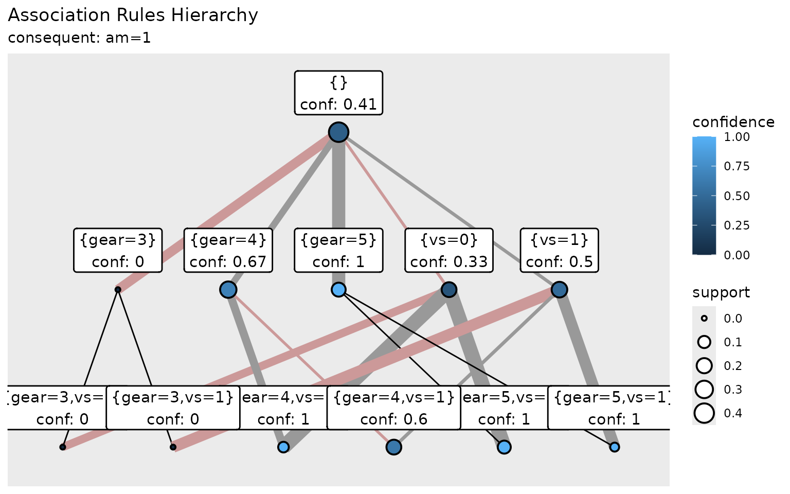
This example creates a hierarchical visualization of association
rules. The geom_diamond() function arranges rules in a
lattice structure where simpler rules (with fewer predicates) appear at
the top and more complex rules below. Visual properties (fill color,
edge width, node size) encode rule quality measures, making it easy to
identify the most interesting patterns. Custom label merges antecedent
with confidence value for better readability. Additional modifications
(scale_x_discrete, scale_y_discrete) add
padding.
The diamond plot helps identify:
- Simple vs. complex rules (vertical position)
- Antecedent relationship (ancestor and descendant rules are connected with lines)
- Strong vs. weak confidence (node color intensity)
- Frequent vs. rare rules (node size)
- Improvement/worsening of confidence (line size and color: improvement is depicted with gray lines, worsening with reddish line; the amount of change is indicated with the width of the lines)
Interactive Exploration
The explore() function launches an interactive Shiny
application for exploring discovered patterns. This is particularly
useful for association rules:
# Search for association rules
rules <- dig_associations(fuzzy_mtcars,
                         antecedent = everything(),
                         consequent = everything(),
                         min_support = 0.05,
                         min_confidence = 0.7)

# Open interactive explorer
explore(rules, data = fuzzy_mtcars)
The interactive explorer provides:
- Rule filtering: Filter rules by support, confidence, lift, and other measures
- Sorting and searching: Find specific rules of interest
- Visualizations: Multiple visualization types for rule exploration
Advanced Use
For advanced workflows, the nuggets package allows users
to define custom pattern types and evaluation functions. This section
demonstrates how to use the general dig() function with
custom callbacks and the specialized dig_grid()
wrapper.
Custom Patterns with dig()
The dig() function allows you to execute a user-defined
callback function on each generated frequent condition. This enables
searching for custom pattern types beyond the pre-defined functions.
The following example replicates the search for association rules using a custom callback function with the datasets prepared earlier:
# Define thresholds for custom association rules
min_support <- 0.02
min_confidence <- 0.8

# Define custom callback function
f <- function(condition, support, pp, pn) {
    # Calculate confidence for each focus (consequent)
    conf <- pp / support

    # Filter rules by confidence and support thresholds
    sel <- !is.na(conf) & conf >= min_confidence & !is.na(pp) & pp >= min_support
    conf <- conf[sel]
    supp <- pp[sel]

    # Return list of rules meeting criteria
    lapply(seq_along(conf), function(i) {
      list(antecedent = format_condition(names(condition)),
           consequent = names(conf)[[i]],
           support = supp[[i]],
           confidence = conf[[i]])
    })
}

# Search using custom callback
custom_result <- dig(fuzzy_mtcars,
                    f = f,
                    condition = !starts_with("am"),
                    focus = starts_with("am"),
                    disjoint = disj,
                    min_length = 1,
                    min_support = min_support)

# Flatten and format results
custom_result <- custom_result |>
  unlist(recursive = FALSE) |>
  lapply(as_tibble) |>
  do.call(rbind, args = _) |>
  arrange(desc(support))

print(custom_result)
#> # A tibble: 5,408 × 4
#>    antecedent              consequent support confidence
#>    <chr>                   <chr>        <dbl>      <dbl>
#>  1 {gear=3}                am=0          15         32
#>  2 {wt=(1.51;3.47;5.42)}   am=0          14.0       22.6
#>  3 {qsec=(14.5;18.7;22.9)} am=0          12.2       19.5
#>  4 {hp=(52;194;335)}       am=0          12.1       24.2
#>  5 {vs=0}                  am=0          12         21.3
#>  6 {gear=3,vs=0}           am=0          12         32
#>  7 {cyl=eight,gear=3,vs=0} am=0          12         32
#>  8 {cyl=eight,vs=0}        am=0          12         27.4
#>  9 {cyl=eight,gear=3}      am=0          12         32
#> 10 {cyl=eight}             am=0          12         27.4
#> # ℹ 5,398 more rows
The callback function f() receives information based on
its argument names:
-
condition: vector of column indices forming the condition -
support: relative frequency of the condition -
pp,pn: contingency table entries
This approach gives you full control over pattern evaluation and filtering logic.
Grid-Based Patterns with dig_grid()
The dig_grid() function is useful for patterns based on
relationships between pairs of columns. It creates a grid of column
combinations and evaluates a user-defined function for each condition
and column pair.
Here’s an example that computes custom statistics for pairs of numeric variables:
# Define callback for grid-based patterns
grid_callback <- function(d, weights) {
    if (nrow(d) < 5) return(NULL)  # Skip if too few observations

    # Compute weighted correlation
    wcor <- cov.wt(d, wt = weights, cor = TRUE)$cor[1, 2]

    list(
        correlation = wcor,
        n_obs = sum(weights > 0.1),
        mean_x = weighted.mean(d[[1]], weights),
        mean_y = weighted.mean(d[[2]], weights)
    )
}

# Prepare combined dataset
combined_fuzzy <- cbind(fuzzy_mtcars, mtcars[, c("mpg", "hp", "wt")])

# Extend disjoint vector for new numeric columns
combined_disj3 <- c(var_names(colnames(fuzzy_mtcars)),
                    c("mpg", "hp", "wt"))

# Search using grid approach
grid_result <- dig_grid(combined_fuzzy,
                       f = grid_callback,
                       condition = colnames(fuzzy_mtcars),
                       xvars = c("mpg", "hp"),
                       yvars = c("wt"),
                       disjoint = combined_disj3,
                       type = "fuzzy",
                       min_length = 1,
                       max_length = 2,
                       min_support = 0.15,
                       max_results = 20)

# Display results
print(grid_result)
#> # A tibble: 40 × 9
#>    condition                                     support xvar  yvar  correlation
#>    <chr>                                           <dbl> <chr> <chr>       <dbl>
#>  1 {qsec=(14.5;18.7;22.9)}                         0.627 mpg   wt         -0.894
#>  2 {qsec=(14.5;18.7;22.9)}                         0.627 hp    wt          0.849
#>  3 {qsec=(14.5;18.7;22.9),wt=(1.51;3.47;5.42)}     0.360 mpg   wt         -0.816
#>  4 {qsec=(14.5;18.7;22.9),wt=(1.51;3.47;5.42)}     0.360 hp    wt          0.710
#>  5 {am=0,qsec=(14.5;18.7;22.9)}                    0.383 mpg   wt         -0.810
#>  6 {am=0,qsec=(14.5;18.7;22.9)}                    0.383 hp    wt          0.759
#>  7 {drat=(2.76;3.84;4.93),qsec=(14.5;18.7;22.9)}   0.341 mpg   wt         -0.850
#>  8 {drat=(2.76;3.84;4.93),qsec=(14.5;18.7;22.9)}   0.341 hp    wt          0.770
#>  9 {qsec=(14.5;18.7;22.9),vs=0}                    0.294 mpg   wt         -0.865
#> 10 {qsec=(14.5;18.7;22.9),vs=0}                    0.294 hp    wt          0.791
#>    n_obs mean_x mean_y condition_length
#>    <int>  <dbl>  <dbl>            <int>
#>  1    29   20.7   3.19                1
#>  2    29  131.    3.19                1
#>  3    24   19.4   3.27                2
#>  4    24  135.    3.27                2
#>  5    18   17.0   3.83                2
#>  6    18  158.    3.83                2
#>  7    26   22.0   2.93                2
#>  8    26  118.    2.93                2
#>  9    16   16.4   3.88                2
#> 10    16  175.    3.88                2
#> # ℹ 30 more rows
The dig_grid() function is particularly useful for:
- Computing conditional correlations with custom methods
- Evaluating pairwise relationships under different conditions
- Implementing specialized statistical tests on variable pairs
Summary
This vignette has introduced the core functionality of the
nuggets package for discovering patterns in data through
systematic exploration of conditions. Key takeaways:
Data Preparation: Transform your data into predicates using
partition().-
Pre-defined Pattern Discovery: The package provides specialized functions for common pattern types:
-
dig_associations()finds association rules (A → C) -
dig_correlations()discovers conditional correlations between variable pairs -
dig_baseline_contrasts()identifies when variables deviate from baseline under conditions -
dig_complement_contrasts()finds subgroups differing from the rest -
dig_paired_baseline_contrasts()compares paired variables within contexts
-
-
Post-processing: Manipulate and visualize discovered patterns:
- Create hierarchical visualizations with
geom_diamond() - Launch interactive explorers with
explore()
- Create hierarchical visualizations with
-
Advanced Usage: Define custom pattern types:
- Use
dig()with custom callback functions for specialized analyses - Use
dig_grid()for patterns based on variable pairs
- Use
Next Steps
- Explore the Data Preparation vignette for advanced preprocessing techniques
- Review function documentation (e.g.,
?dig_associations) for detailed parameter descriptions - Experiment with your own datasets to discover meaningful patterns
- Use interactive exploration (
explore()) to gain insights into discovered patterns
The nuggets package provides a flexible framework for
pattern discovery that scales from simple association rule mining to
complex custom pattern searches, all while supporting both crisp and
fuzzy logic approaches.