Introduction
Before applying nuggets for pattern discovery, data
columns intended as predicates must be prepared either by
dichotomization (conversion into dummy variables) or
by transformation into fuzzy sets. This vignette provides a
comprehensive guide to data preparation functions and techniques
available in the nuggets package.
The package provides two main approaches for data preparation:
Crisp (Boolean) predicates: Transform data columns into logical (
TRUE/FALSE) columns. This approach is simpler and faster, and is recommended for most applications.Fuzzy predicates: Transform numeric columns into membership degrees in the interval \([0, 1]\). This approach is more flexible and allows modeling of uncertainty in data, but is more computationally demanding.
The primary function for data preparation is
partition(), which handles both crisp and fuzzy
transformations. Additional utility functions help identify and remove
uninformative columns and detect tautologies in the data.
Data Preparation with partition()
For patterns based on crisp conditions, the data columns that serve
as predicates in conditions must be transformed either to logical
(TRUE/FALSE) columns, or to fuzzy sets with
values from the interval \([0, 1]\).
The first option is simpler and faster, and it is the recommended option
for most applications. The second option is more flexible and allows to
model uncertainty in data, but it is more computationally demanding.
Preparation of Crisp (Boolean) Predicates
For patterns based on crisp conditions, the data columns that would
serve as predicates in conditions have to be transformed to logical
(TRUE/FALSE) columns. That can be done in two
ways:
- numeric columns can be transformed to factors with a selected number of levels, and then
- factors can be transformed to dummy logical columns.
Both operations can be done with the help of the
partition() function. The partition() function
requires the dataset as its first argument and a tidyselect
selection expression to select the columns to be transformed.
Factors and logical columns are automatically transformed to dummy
logical columns by the partition() function. For numeric
columns, the partition() function requires the
.method argument to specify the method of partitioning:
-
.method = "dummy"transforms numeric columns to factors and then to dummy logical columns. That effectively creates a separate logical column for each distinct value of the numeric column. -
.method = "crisp"transforms numeric columns to crisp predicates by dividing the range of values into intervals and coding the values into dummy logical columns according to the intervals. - there exist other methods of partitioning of numeric columns. These methods create fuzzy predicates and are described in the next section.
For example, consider the built-in mtcars dataset. This
dataset contains information about various car models. For the sake of
illustration, let us transform the cyl column into factor
first:
# Create a copy to avoid modifying the original dataset
mtcars_example <- mtcars
mtcars_example$cyl <- factor(mtcars_example$cyl,
                     levels= c(4, 6, 8),
                     labels = c("four", "six", "eight"))
head(mtcars_example)
#>                    mpg   cyl disp  hp drat    wt  qsec vs am gear carb
#> Mazda RX4         21.0   six  160 110 3.90 2.620 16.46  0  1    4    4
#> Mazda RX4 Wag     21.0   six  160 110 3.90 2.875 17.02  0  1    4    4
#> Datsun 710        22.8  four  108  93 3.85 2.320 18.61  1  1    4    1
#> Hornet 4 Drive    21.4   six  258 110 3.08 3.215 19.44  1  0    3    1
#> Hornet Sportabout 18.7 eight  360 175 3.15 3.440 17.02  0  0    3    2
#> Valiant           18.1   six  225 105 2.76 3.460 20.22  1  0    3    1
Factors are transformed to dummy logical columns by the
partition() function automatically:
partition(mtcars_example, cyl)
#> # A tibble: 32 × 13
#>      mpg  disp    hp  drat    wt  qsec    vs    am  gear  carb `cyl=four`
#>    <dbl> <dbl> <dbl> <dbl> <dbl> <dbl> <dbl> <dbl> <dbl> <dbl> <lgl>
#>  1  21    160    110  3.9   2.62  16.5     0     1     4     4 FALSE
#>  2  21    160    110  3.9   2.88  17.0     0     1     4     4 FALSE
#>  3  22.8  108     93  3.85  2.32  18.6     1     1     4     1 TRUE
#>  4  21.4  258    110  3.08  3.22  19.4     1     0     3     1 FALSE
#>  5  18.7  360    175  3.15  3.44  17.0     0     0     3     2 FALSE
#>  6  18.1  225    105  2.76  3.46  20.2     1     0     3     1 FALSE
#>  7  14.3  360    245  3.21  3.57  15.8     0     0     3     4 FALSE
#>  8  24.4  147.    62  3.69  3.19  20       1     0     4     2 TRUE
#>  9  22.8  141.    95  3.92  3.15  22.9     1     0     4     2 TRUE
#> 10  19.2  168.   123  3.92  3.44  18.3     1     0     4     4 FALSE
#>    `cyl=six` `cyl=eight`
#>    <lgl>     <lgl>
#>  1 TRUE      FALSE
#>  2 TRUE      FALSE
#>  3 FALSE     FALSE
#>  4 TRUE      FALSE
#>  5 FALSE     TRUE
#>  6 TRUE      FALSE
#>  7 FALSE     TRUE
#>  8 FALSE     FALSE
#>  9 FALSE     FALSE
#> 10 TRUE      FALSE
#> # ℹ 22 more rows
The vs, am, and gear columns
are numeric but actually represent categories. To transform them to
dummy logical columns in the same way as factors, we can use the
partition() function with the .method argument
set to "dummy":
partition(mtcars_example, vs:gear, .method = "dummy")
#> # A tibble: 32 × 15
#>      mpg cyl    disp    hp  drat    wt  qsec  carb `vs=0` `vs=1` `am=0` `am=1`
#>    <dbl> <fct> <dbl> <dbl> <dbl> <dbl> <dbl> <dbl> <lgl>  <lgl>  <lgl>  <lgl>
#>  1  21   six    160    110  3.9   2.62  16.5     4 TRUE   FALSE  FALSE  TRUE
#>  2  21   six    160    110  3.9   2.88  17.0     4 TRUE   FALSE  FALSE  TRUE
#>  3  22.8 four   108     93  3.85  2.32  18.6     1 FALSE  TRUE   FALSE  TRUE
#>  4  21.4 six    258    110  3.08  3.22  19.4     1 FALSE  TRUE   TRUE   FALSE
#>  5  18.7 eight  360    175  3.15  3.44  17.0     2 TRUE   FALSE  TRUE   FALSE
#>  6  18.1 six    225    105  2.76  3.46  20.2     1 FALSE  TRUE   TRUE   FALSE
#>  7  14.3 eight  360    245  3.21  3.57  15.8     4 TRUE   FALSE  TRUE   FALSE
#>  8  24.4 four   147.    62  3.69  3.19  20       2 FALSE  TRUE   TRUE   FALSE
#>  9  22.8 four   141.    95  3.92  3.15  22.9     2 FALSE  TRUE   TRUE   FALSE
#> 10  19.2 six    168.   123  3.92  3.44  18.3     4 FALSE  TRUE   TRUE   FALSE
#>    `gear=3` `gear=4` `gear=5`
#>    <lgl>    <lgl>    <lgl>
#>  1 FALSE    TRUE     FALSE
#>  2 FALSE    TRUE     FALSE
#>  3 FALSE    TRUE     FALSE
#>  4 TRUE     FALSE    FALSE
#>  5 TRUE     FALSE    FALSE
#>  6 TRUE     FALSE    FALSE
#>  7 TRUE     FALSE    FALSE
#>  8 FALSE    TRUE     FALSE
#>  9 FALSE    TRUE     FALSE
#> 10 FALSE    TRUE     FALSE
#> # ℹ 22 more rows
The mpg column is numeric and therefore cannot be
transformed directly into dummy logical columns. A better approach is to
use the "crisp" method of partitioning.
The "crisp" method divides the range of values of the
selected columns into intervals specified by the .breaks
argument and then encodes the values into dummy logical columns
corresponding to the intervals. The .breaks argument is a
numeric vector that specifies the interval boundaries.
For example, the mpg values can be divided into four
intervals: (-Inf, 15], (15, 20], (20, 30], and (30, Inf). The
.breaks argument is then the vector
c(-Inf, 15, 20, 30, Inf), which defines the boundaries of
these intervals.
partition(mtcars_example, mpg, .method = "crisp", .breaks = c(-Inf, 15, 20, 30, Inf))
#> # A tibble: 32 × 14
#>    cyl    disp    hp  drat    wt  qsec    vs    am  gear  carb `mpg=(-Inf;15]`
#>    <fct> <dbl> <dbl> <dbl> <dbl> <dbl> <dbl> <dbl> <dbl> <dbl> <lgl>
#>  1 six    160    110  3.9   2.62  16.5     0     1     4     4 FALSE
#>  2 six    160    110  3.9   2.88  17.0     0     1     4     4 FALSE
#>  3 four   108     93  3.85  2.32  18.6     1     1     4     1 FALSE
#>  4 six    258    110  3.08  3.22  19.4     1     0     3     1 FALSE
#>  5 eight  360    175  3.15  3.44  17.0     0     0     3     2 FALSE
#>  6 six    225    105  2.76  3.46  20.2     1     0     3     1 FALSE
#>  7 eight  360    245  3.21  3.57  15.8     0     0     3     4 TRUE
#>  8 four   147.    62  3.69  3.19  20       1     0     4     2 FALSE
#>  9 four   141.    95  3.92  3.15  22.9     1     0     4     2 FALSE
#> 10 six    168.   123  3.92  3.44  18.3     1     0     4     4 FALSE
#>    `mpg=(15;20]` `mpg=(20;30]` `mpg=(30;Inf]`
#>    <lgl>         <lgl>         <lgl>
#>  1 FALSE         TRUE          FALSE
#>  2 FALSE         TRUE          FALSE
#>  3 FALSE         TRUE          FALSE
#>  4 FALSE         TRUE          FALSE
#>  5 TRUE          FALSE         FALSE
#>  6 TRUE          FALSE         FALSE
#>  7 FALSE         FALSE         FALSE
#>  8 FALSE         TRUE          FALSE
#>  9 FALSE         TRUE          FALSE
#> 10 TRUE          FALSE         FALSE
#> # ℹ 22 more rows
Note: it is advisable to put -Inf and Inf
as the first and last elements of the .breaks vector to
ensure that all values are covered by the intervals.
If we want the breaks to be evenly spaced across the range of values,
we can set .breaks to a single integer. This value
specifies the number of intervals to create. For example, the following
command divides the disp values into three intervals of
equal width:
partition(mtcars_example, disp, .method = "crisp", .breaks = 3)
#> # A tibble: 32 × 13
#>      mpg cyl      hp  drat    wt  qsec    vs    am  gear  carb `disp=(-Inf;205]`
#>    <dbl> <fct> <dbl> <dbl> <dbl> <dbl> <dbl> <dbl> <dbl> <dbl> <lgl>
#>  1  21   six     110  3.9   2.62  16.5     0     1     4     4 TRUE
#>  2  21   six     110  3.9   2.88  17.0     0     1     4     4 TRUE
#>  3  22.8 four     93  3.85  2.32  18.6     1     1     4     1 TRUE
#>  4  21.4 six     110  3.08  3.22  19.4     1     0     3     1 FALSE
#>  5  18.7 eight   175  3.15  3.44  17.0     0     0     3     2 FALSE
#>  6  18.1 six     105  2.76  3.46  20.2     1     0     3     1 FALSE
#>  7  14.3 eight   245  3.21  3.57  15.8     0     0     3     4 FALSE
#>  8  24.4 four     62  3.69  3.19  20       1     0     4     2 TRUE
#>  9  22.8 four     95  3.92  3.15  22.9     1     0     4     2 TRUE
#> 10  19.2 six     123  3.92  3.44  18.3     1     0     4     4 TRUE
#>    `disp=(205;338]` `disp=(338;Inf]`
#>    <lgl>            <lgl>
#>  1 FALSE            FALSE
#>  2 FALSE            FALSE
#>  3 FALSE            FALSE
#>  4 TRUE             FALSE
#>  5 FALSE            TRUE
#>  6 TRUE             FALSE
#>  7 FALSE            TRUE
#>  8 FALSE            FALSE
#>  9 FALSE            FALSE
#> 10 FALSE            FALSE
#> # ℹ 22 more rows
Each call to partition() returns a tibble with the
selected columns transformed to dummy logical columns, while the other
columns remain unchanged.
The transformation of the whole mtcars dataset to crisp
predicates can be done as follows:
crisp_mtcars <- mtcars_example |>
    partition(cyl, vs:gear, .method = "dummy") |>
    partition(mpg, .method = "crisp", .breaks = c(-Inf, 15, 20, 30, Inf)) |>
    partition(disp:carb, .method = "crisp", .breaks = 3)

head(crisp_mtcars, n = 3)
#> # A tibble: 3 × 32
#>   `cyl=four` `cyl=six` `cyl=eight` `vs=0` `vs=1` `am=0` `am=1` `gear=3` `gear=4`
#>   <lgl>      <lgl>     <lgl>       <lgl>  <lgl>  <lgl>  <lgl>  <lgl>    <lgl>
#> 1 FALSE      TRUE      FALSE       TRUE   FALSE  FALSE  TRUE   FALSE    TRUE
#> 2 FALSE      TRUE      FALSE       TRUE   FALSE  FALSE  TRUE   FALSE    TRUE
#> 3 TRUE       FALSE     FALSE       FALSE  TRUE   FALSE  TRUE   FALSE    TRUE
#>   `gear=5` `mpg=(-Inf;15]` `mpg=(15;20]` `mpg=(20;30]` `mpg=(30;Inf]`
#>   <lgl>    <lgl>           <lgl>         <lgl>         <lgl>
#> 1 FALSE    FALSE           FALSE         TRUE          FALSE
#> 2 FALSE    FALSE           FALSE         TRUE          FALSE
#> 3 FALSE    FALSE           FALSE         TRUE          FALSE
#>   `disp=(-Inf;205]` `disp=(205;338]` `disp=(338;Inf]` `hp=(-Inf;146]`
#>   <lgl>             <lgl>            <lgl>            <lgl>
#> 1 TRUE              FALSE            FALSE            TRUE
#> 2 TRUE              FALSE            FALSE            TRUE
#> 3 TRUE              FALSE            FALSE            TRUE
#>   `hp=(146;241]` `hp=(241;Inf]` `drat=(-Inf;3.48]` `drat=(3.48;4.21]`
#>   <lgl>          <lgl>          <lgl>              <lgl>
#> 1 FALSE          FALSE          FALSE              TRUE
#> 2 FALSE          FALSE          FALSE              TRUE
#> 3 FALSE          FALSE          FALSE              TRUE
#>   `drat=(4.21;Inf]` `wt=(-Inf;2.82]` `wt=(2.82;4.12]` `wt=(4.12;Inf]`
#>   <lgl>             <lgl>            <lgl>            <lgl>
#> 1 FALSE             TRUE             FALSE            FALSE
#> 2 FALSE             FALSE            TRUE             FALSE
#> 3 FALSE             TRUE             FALSE            FALSE
#>   `qsec=(-Inf;17.3]` `qsec=(17.3;20.1]` `qsec=(20.1;Inf]` `carb=(-Inf;3.33]`
#>   <lgl>              <lgl>              <lgl>             <lgl>
#> 1 TRUE               FALSE              FALSE             FALSE
#> 2 TRUE               FALSE              FALSE             FALSE
#> 3 FALSE              TRUE               FALSE             TRUE
#>   `carb=(3.33;5.67]` `carb=(5.67;Inf]`
#>   <lgl>              <lgl>
#> 1 TRUE               FALSE
#> 2 TRUE               FALSE
#> 3 FALSE              FALSE
Now all columns are logical and can be used as predicates in crisp conditions.
Data-Driven Breakpoint Selection with .style
When .breaks is specified as a single integer (the
number of intervals), the partition() function can use
various data-driven methods to determine optimal breakpoints, rather
than simply dividing the range into equal-width intervals. This is
controlled by the .style argument, which leverages methods
from the classInt package.
The .style argument supports the following methods:
-
"equal"(default) – equal-width intervals across the column range -
"quantile"– equal-frequency intervals (quantile-based) -
"kmeans"– intervals found by 1D k-means clustering -
"sd"– intervals based on standard deviations from the mean -
"hclust"– hierarchical clustering intervals -
"bclust"– model-based clustering intervals -
"fisher"/"jenks"– Fisher–Jenks optimal partitioning -
"dpih"– kernel-based density partitioning -
"headtails"– head/tails natural breaks -
"maximum"– maximization-based partitioning -
"box"– breaks at boxplot hinges
These methods are particularly useful when the data distribution is skewed or has natural clusters. For example, quantile-based partitioning ensures that each interval contains approximately the same number of observations, which can be valuable for imbalanced datasets.
Here are examples using the CO2 dataset:
# Equal-width intervals (default)
partition(CO2, conc, .method = "crisp", .breaks = 4, .style = "equal")
#> # A tibble: 84 × 8
#>    Plant Type   Treatment  uptake `conc=(-Inf;321]` `conc=(321;548]`
#>    <ord> <fct>  <fct>       <dbl> <lgl>             <lgl>
#>  1 Qn1   Quebec nonchilled   16   TRUE              FALSE
#>  2 Qn1   Quebec nonchilled   30.4 TRUE              FALSE
#>  3 Qn1   Quebec nonchilled   34.8 TRUE              FALSE
#>  4 Qn1   Quebec nonchilled   37.2 FALSE             TRUE
#>  5 Qn1   Quebec nonchilled   35.3 FALSE             TRUE
#>  6 Qn1   Quebec nonchilled   39.2 FALSE             FALSE
#>  7 Qn1   Quebec nonchilled   39.7 FALSE             FALSE
#>  8 Qn2   Quebec nonchilled   13.6 TRUE              FALSE
#>  9 Qn2   Quebec nonchilled   27.3 TRUE              FALSE
#> 10 Qn2   Quebec nonchilled   37.1 TRUE              FALSE
#>    `conc=(548;774]` `conc=(774;Inf]`
#>    <lgl>            <lgl>
#>  1 FALSE            FALSE
#>  2 FALSE            FALSE
#>  3 FALSE            FALSE
#>  4 FALSE            FALSE
#>  5 FALSE            FALSE
#>  6 TRUE             FALSE
#>  7 FALSE            TRUE
#>  8 FALSE            FALSE
#>  9 FALSE            FALSE
#> 10 FALSE            FALSE
#> # ℹ 74 more rows
# Quantile-based intervals (equal frequency in each interval)
partition(CO2, conc, .method = "crisp", .breaks = 4, .style = "quantile")
#> # A tibble: 84 × 8
#>    Plant Type   Treatment  uptake `conc=(-Inf;175]` `conc=(175;350]`
#>    <ord> <fct>  <fct>       <dbl> <lgl>             <lgl>
#>  1 Qn1   Quebec nonchilled   16   TRUE              FALSE
#>  2 Qn1   Quebec nonchilled   30.4 TRUE              FALSE
#>  3 Qn1   Quebec nonchilled   34.8 FALSE             TRUE
#>  4 Qn1   Quebec nonchilled   37.2 FALSE             TRUE
#>  5 Qn1   Quebec nonchilled   35.3 FALSE             FALSE
#>  6 Qn1   Quebec nonchilled   39.2 FALSE             FALSE
#>  7 Qn1   Quebec nonchilled   39.7 FALSE             FALSE
#>  8 Qn2   Quebec nonchilled   13.6 TRUE              FALSE
#>  9 Qn2   Quebec nonchilled   27.3 TRUE              FALSE
#> 10 Qn2   Quebec nonchilled   37.1 FALSE             TRUE
#>    `conc=(350;675]` `conc=(675;Inf]`
#>    <lgl>            <lgl>
#>  1 FALSE            FALSE
#>  2 FALSE            FALSE
#>  3 FALSE            FALSE
#>  4 FALSE            FALSE
#>  5 TRUE             FALSE
#>  6 TRUE             FALSE
#>  7 FALSE            TRUE
#>  8 FALSE            FALSE
#>  9 FALSE            FALSE
#> 10 FALSE            FALSE
#> # ℹ 74 more rows
# K-means clustering to find natural breakpoints
partition(CO2, conc, .method = "crisp", .breaks = 4, .style = "kmeans")
#> # A tibble: 84 × 8
#>    Plant Type   Treatment  uptake `conc=(-Inf;212]` `conc=(212;425]`
#>    <ord> <fct>  <fct>       <dbl> <lgl>             <lgl>
#>  1 Qn1   Quebec nonchilled   16   TRUE              FALSE
#>  2 Qn1   Quebec nonchilled   30.4 TRUE              FALSE
#>  3 Qn1   Quebec nonchilled   34.8 FALSE             TRUE
#>  4 Qn1   Quebec nonchilled   37.2 FALSE             TRUE
#>  5 Qn1   Quebec nonchilled   35.3 FALSE             FALSE
#>  6 Qn1   Quebec nonchilled   39.2 FALSE             FALSE
#>  7 Qn1   Quebec nonchilled   39.7 FALSE             FALSE
#>  8 Qn2   Quebec nonchilled   13.6 TRUE              FALSE
#>  9 Qn2   Quebec nonchilled   27.3 TRUE              FALSE
#> 10 Qn2   Quebec nonchilled   37.1 FALSE             TRUE
#>    `conc=(425;838]` `conc=(838;Inf]`
#>    <lgl>            <lgl>
#>  1 FALSE            FALSE
#>  2 FALSE            FALSE
#>  3 FALSE            FALSE
#>  4 FALSE            FALSE
#>  5 TRUE             FALSE
#>  6 TRUE             FALSE
#>  7 FALSE            TRUE
#>  8 FALSE            FALSE
#>  9 FALSE            FALSE
#> 10 FALSE            FALSE
#> # ℹ 74 more rows
# Standard deviation-based intervals
partition(CO2, conc, .method = "crisp", .breaks = 4, .style = "sd")
#> # A tibble: 84 × 8
#>    Plant Type   Treatment  uptake `conc=(-Inf;139]` `conc=(139;435]`
#>    <ord> <fct>  <fct>       <dbl> <lgl>             <lgl>
#>  1 Qn1   Quebec nonchilled   16   TRUE              FALSE
#>  2 Qn1   Quebec nonchilled   30.4 FALSE             TRUE
#>  3 Qn1   Quebec nonchilled   34.8 FALSE             TRUE
#>  4 Qn1   Quebec nonchilled   37.2 FALSE             TRUE
#>  5 Qn1   Quebec nonchilled   35.3 FALSE             FALSE
#>  6 Qn1   Quebec nonchilled   39.2 FALSE             FALSE
#>  7 Qn1   Quebec nonchilled   39.7 FALSE             FALSE
#>  8 Qn2   Quebec nonchilled   13.6 TRUE              FALSE
#>  9 Qn2   Quebec nonchilled   27.3 FALSE             TRUE
#> 10 Qn2   Quebec nonchilled   37.1 FALSE             TRUE
#>    `conc=(435;731]` `conc=(731;Inf]`
#>    <lgl>            <lgl>
#>  1 FALSE            FALSE
#>  2 FALSE            FALSE
#>  3 FALSE            FALSE
#>  4 FALSE            FALSE
#>  5 TRUE             FALSE
#>  6 TRUE             FALSE
#>  7 FALSE            TRUE
#>  8 FALSE            FALSE
#>  9 FALSE            FALSE
#> 10 FALSE            FALSE
#> # ℹ 74 more rows
The .style_params argument allows you to pass additional
parameters to the underlying algorithm. This should be a named list of
arguments accepted by the respective method in
classInt::classIntervals().
For example, when using k-means clustering, you can specify the algorithm:
# Use Lloyd's algorithm for k-means
partition(CO2, conc, .method = "crisp", .breaks = 4,
          .style = "kmeans",
          .style_params = list(algorithm = "Lloyd"))
#> # A tibble: 84 × 8
#>    Plant Type   Treatment  uptake `conc=(-Inf;300]` `conc=(300;588]`
#>    <ord> <fct>  <fct>       <dbl> <lgl>             <lgl>
#>  1 Qn1   Quebec nonchilled   16   TRUE              FALSE
#>  2 Qn1   Quebec nonchilled   30.4 TRUE              FALSE
#>  3 Qn1   Quebec nonchilled   34.8 TRUE              FALSE
#>  4 Qn1   Quebec nonchilled   37.2 FALSE             TRUE
#>  5 Qn1   Quebec nonchilled   35.3 FALSE             TRUE
#>  6 Qn1   Quebec nonchilled   39.2 FALSE             FALSE
#>  7 Qn1   Quebec nonchilled   39.7 FALSE             FALSE
#>  8 Qn2   Quebec nonchilled   13.6 TRUE              FALSE
#>  9 Qn2   Quebec nonchilled   27.3 TRUE              FALSE
#> 10 Qn2   Quebec nonchilled   37.1 TRUE              FALSE
#>    `conc=(588;838]` `conc=(838;Inf]`
#>    <lgl>            <lgl>
#>  1 FALSE            FALSE
#>  2 FALSE            FALSE
#>  3 FALSE            FALSE
#>  4 FALSE            FALSE
#>  5 FALSE            FALSE
#>  6 TRUE             FALSE
#>  7 FALSE            TRUE
#>  8 FALSE            FALSE
#>  9 FALSE            FALSE
#> 10 FALSE            FALSE
#> # ℹ 74 more rows
When using quantile-based intervals, you can control the quantile type:
# Use different quantile types (see ?quantile for details)
partition(CO2, conc, .method = "crisp", .breaks = 4,
          .style = "quantile",
          .style_params = list(type = 7))
#> # A tibble: 84 × 8
#>    Plant Type   Treatment  uptake `conc=(-Inf;175]` `conc=(175;350]`
#>    <ord> <fct>  <fct>       <dbl> <lgl>             <lgl>
#>  1 Qn1   Quebec nonchilled   16   TRUE              FALSE
#>  2 Qn1   Quebec nonchilled   30.4 TRUE              FALSE
#>  3 Qn1   Quebec nonchilled   34.8 FALSE             TRUE
#>  4 Qn1   Quebec nonchilled   37.2 FALSE             TRUE
#>  5 Qn1   Quebec nonchilled   35.3 FALSE             FALSE
#>  6 Qn1   Quebec nonchilled   39.2 FALSE             FALSE
#>  7 Qn1   Quebec nonchilled   39.7 FALSE             FALSE
#>  8 Qn2   Quebec nonchilled   13.6 TRUE              FALSE
#>  9 Qn2   Quebec nonchilled   27.3 TRUE              FALSE
#> 10 Qn2   Quebec nonchilled   37.1 FALSE             TRUE
#>    `conc=(350;675]` `conc=(675;Inf]`
#>    <lgl>            <lgl>
#>  1 FALSE            FALSE
#>  2 FALSE            FALSE
#>  3 FALSE            FALSE
#>  4 FALSE            FALSE
#>  5 TRUE             FALSE
#>  6 TRUE             FALSE
#>  7 FALSE            TRUE
#>  8 FALSE            FALSE
#>  9 FALSE            FALSE
#> 10 FALSE            FALSE
#> # ℹ 74 more rows
These data-driven methods can produce more meaningful intervals that better reflect the structure of your data, leading to more interpretable patterns in subsequent analysis.
Preparation of Triangular and Raised-Cosine Fuzzy Predicates
In many real-world datasets, numeric attributes do not lend themselves to clear-cut, crisp boundaries. For example, deciding whether a car has “low mileage” or “high mileage” is often subjective. A vehicle with 19 miles per gallon may be considered “low” in one context but “medium” in another. Crisp intervals force a strict separation between categories, which can be too rigid and may lose information about gradual changes in the data.
To address this, fuzzy predicates are used. A fuzzy
predicate expresses the degree to which a condition is satisfied.
Instead of being strictly TRUE or FALSE
(although allowed too), each predicate is represented by a number in the
interval \([0,1]\). A truth degree of 0
means the predicate is entirely false, 1 means it is fully true, and
values in between indicate partial membership. This allows us to model
smooth transitions between categories and capture more nuanced
patterns.
For example, a fuzzy predicate could represent “medium horsepower” in
the mtcars dataset. A car with 120 hp may belong to this
category to a degree of 0.8, while a car with 150 hp may belong to it
only to a degree of 0.2. Such representations are more faithful to human
reasoning and often yield patterns that are both more robust and more
interpretable.
The transformation of numeric columns to fuzzy predicates can be done
with the partition() function. As with crisp partitioning,
factors are transformed to dummy logical columns. Numeric columns,
however, are transformed into fuzzy truth values. The
partition() function provides two fuzzy partitioning
methods:
-
.method = "triangle"creates fuzzy sets with triangular or trapezoidal membership functions; -
.method = "raisedcos"creates fuzzy sets with raised cosine or trapezoidal raised-cosine membership functions.
These membership functions specify how strongly a value belongs to a fuzzy set. The choice of function depends on the desired smoothness of the transition between sets.
More advanced fuzzy partitioning of numeric columns can be achieved with the lfl package, which provides tools for defining fuzzy sets of many types, including linguistic terms such as “very small” or “extremely big”. See the
lfldocumentation for more information.
Both triangular and raised cosine shapes are fully defined by three
points: the left border, the peak, and the right border. The
.breaks argument in the partition() function
specifies these points. See the following figure for an illustration of
triangular and raised cosine membership functions for
.breaks = c(-10, 0, 10):
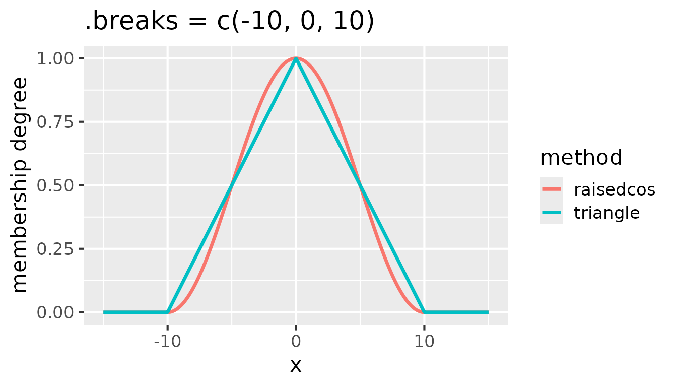
Comparison of triangular and raised cosine membership functions for
.breaks = c(-10, 0, 10)
Each consecutive triplet of values in .breaks defines
one fuzzy set. To create e.g. three fuzzy sets, five break points are
needed. For instance, .breaks = c(-10, -5, 0, 5, 10)
defines three fuzzy sets with peaks at -5, 0, and 5. See the following
figure for an illustration of these fuzzy sets:
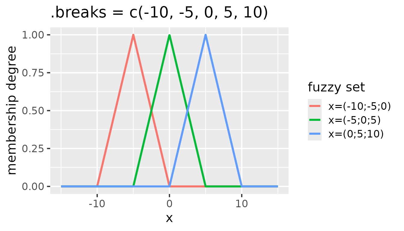
Fuzzy sets with triangular membership functions for
partition(x, .method = "triangle", .breaks = c(-10, -5, 0, 5, 10))
It is often useful to extend the fuzzy sets on the edges to infinity.
That ensures that all values are covered by the fuzzy sets. To achieve
that, -Inf and Inf can be added as the first
and last elements of the .breaks vector:
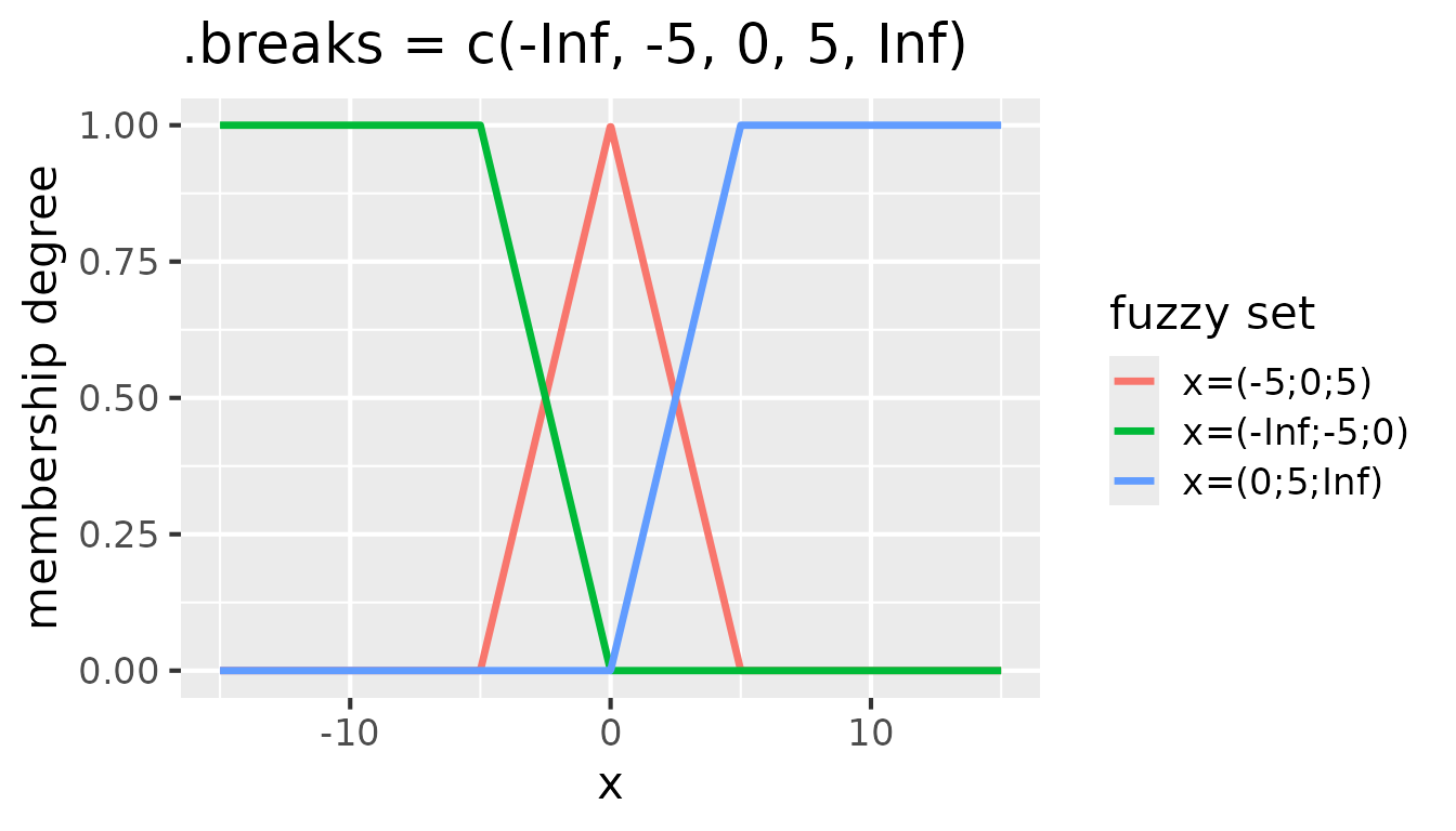
Fuzzy sets with triangular membership functions for
partition(x, .method = "triangle", .breaks = c(-Inf, -5, 0, 5, Inf))
If a regular partitioning of the range of values is desired,
.breaks can be set to a single integer, which specifies the
number of fuzzy sets to create. For example, .breaks = 4
creates partitioning with four fuzzy sets:
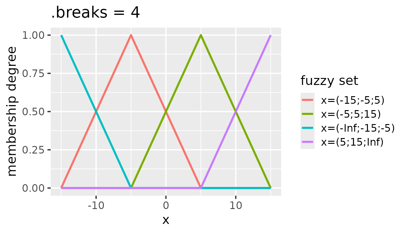
Fuzzy sets with triangular membership functions for
partition(x, .method = "triangle", .breaks = 4)
The same is valid for raised cosine fuzzy sets. For instance, the
following figure shows five raised cosine fuzzy sets defined by
.breaks = c(-Inf, -10, -5, 0, 5, 10, Inf):
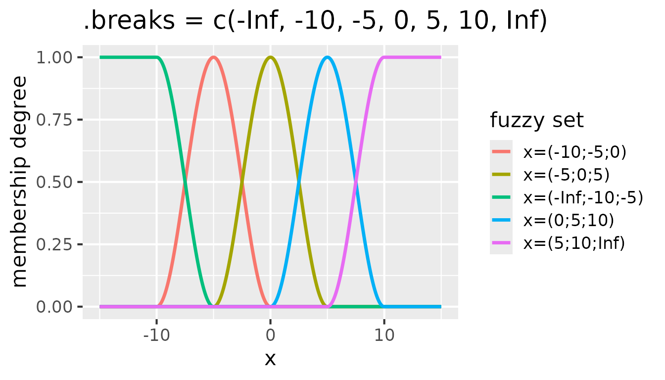
Fuzzy sets with raised cosine membership functions for
partition(x, .method = "raisedcos", .breaks = c(-Inf, -10, -5, 0, 5, 10, Inf))
A fuzzy transformation of the whole mtcars dataset can
be done as follows:
# Start with a fresh copy of mtcars
fuzzy_mtcars <- mtcars |>
    mutate(cyl = factor(cyl, levels = c(4, 6, 8), labels = c("four", "six", "eight"))) |>
    partition(cyl, vs:gear, .method = "dummy") |>
    partition(mpg, .method = "triangle", .breaks = c(-Inf, 15, 20, 30, Inf)) |>
    partition(disp:carb, .method = "triangle", .breaks = 3)

head(fuzzy_mtcars, n = 3)
#> # A tibble: 3 × 31
#>   `cyl=four` `cyl=six` `cyl=eight` `vs=0` `vs=1` `am=0` `am=1` `gear=3` `gear=4`
#>   <lgl>      <lgl>     <lgl>       <lgl>  <lgl>  <lgl>  <lgl>  <lgl>    <lgl>
#> 1 FALSE      TRUE      FALSE       TRUE   FALSE  FALSE  TRUE   FALSE    TRUE
#> 2 FALSE      TRUE      FALSE       TRUE   FALSE  FALSE  TRUE   FALSE    TRUE
#> 3 TRUE       FALSE     FALSE       FALSE  TRUE   FALSE  TRUE   FALSE    TRUE
#>   `gear=5` `mpg=(-Inf;15;20)` `mpg=(15;20;30)` `mpg=(20;30;Inf)`
#>   <lgl>                 <dbl>            <dbl>             <dbl>
#> 1 FALSE                     0             0.9               0.1
#> 2 FALSE                     0             0.9               0.1
#> 3 FALSE                     0             0.72              0.28
#>   `disp=(-Inf;71.1;272)` `disp=(71.1;272;472)` `disp=(272;472;Inf)`
#>                    <dbl>                 <dbl>                <dbl>
#> 1                  0.557                 0.443                    0
#> 2                  0.557                 0.443                    0
#> 3                  0.816                 0.184                    0
#>   `hp=(-Inf;52;194)` `hp=(52;194;335)` `hp=(194;335;Inf)`
#>                <dbl>             <dbl>              <dbl>
#> 1              0.592             0.408                  0
#> 2              0.592             0.408                  0
#> 3              0.711             0.289                  0
#>   `drat=(-Inf;2.76;3.84)` `drat=(2.76;3.84;4.93)` `drat=(3.84;4.93;Inf)`
#>                     <dbl>                   <dbl>                  <dbl>
#> 1                       0                   0.945                0.0550
#> 2                       0                   0.945                0.0550
#> 3                       0                   0.991                0.00917
#>   `wt=(-Inf;1.51;3.47)` `wt=(1.51;3.47;5.42)` `wt=(3.47;5.42;Inf)`
#>                   <dbl>                 <dbl>                <dbl>
#> 1                 0.434                 0.566                    0
#> 2                 0.304                 0.696                    0
#> 3                 0.587                 0.413                    0
#>   `qsec=(-Inf;14.5;18.7)` `qsec=(14.5;18.7;22.9)` `qsec=(18.7;22.9;Inf)`
#>                     <dbl>                   <dbl>                  <dbl>
#> 1                  0.533                    0.467                      0
#> 2                  0.4                      0.6                        0
#> 3                  0.0214                   0.979                      0
#>   `carb=(-Inf;1;4.5)` `carb=(1;4.5;8)` `carb=(4.5;8;Inf)`
#>                 <dbl>            <dbl>              <dbl>
#> 1               0.143            0.857                  0
#> 2               0.143            0.857                  0
#> 3               1                0                      0
Note that the cyl, vs, am, and
gear columns are still represented by dummy logical
columns, while the mpg, disp, and other
columns are now represented by fuzzy sets. This combination allows both
crisp and fuzzy predicates to be used together in pattern discovery,
offering more flexibility and interpretability.
Preparation of Trapezoidal Fuzzy Predicates
The triangular and raised cosine membership functions are often sufficient to capture gradual transitions in numeric data. However, in some situations it is useful to have fuzzy sets that stay fully true (membership = 1) over a wider interval before decreasing again. This generalization corresponds to a trapezoidal fuzzy set, which can be seen as a triangle or raised cosine with a “flat top”.
With partition(), trapezoids can be defined for both
"triangle" and "raisedcos" methods by
controlling how many consecutive break points constitute one fuzzy set
and how far the window shifts along the breaks. That can be accomplished
with the .span and .inc arguments:
-
.span- specifies the width of the flat top in terms of the number of break intervals that should be merged. -
.inc- the shift of the window along.breakswhen forming the next fuzzy set.
By default, .span = 1 and .inc = 1, which
means that each fuzzy set is triangular or raised cosine. Setting
.span to a value greater than 1 creates trapezoidal fuzzy
sets. With .span = 2, each fuzzy set is defined by four
consecutive break points - a flat top spans two break intervals. The
following figure is the result of setting .span = 2 and
.breaks = c(-10, -5, 5, 10):
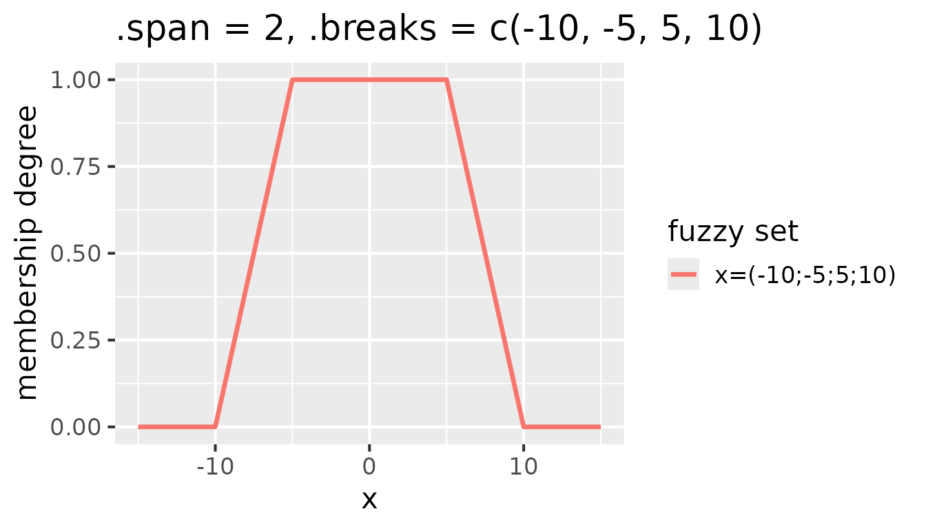
Fuzzy sets with triangular membership functions for
partition(x, .method = "triangle", .span = 2, .breaks = c(-10, -5, 5, 10))
Additional fuzzy sets are created by shifting the window along the
break points. The shift is controlled by the .inc argument.
By default, .inc = 1, which means that the window shifts by
one break point. Consider the following example that shows the effect of
setting .inc = 1 in addition to .span = 2 and
.breaks = c(-15, -10, -5, 0, 5, 10, 15):
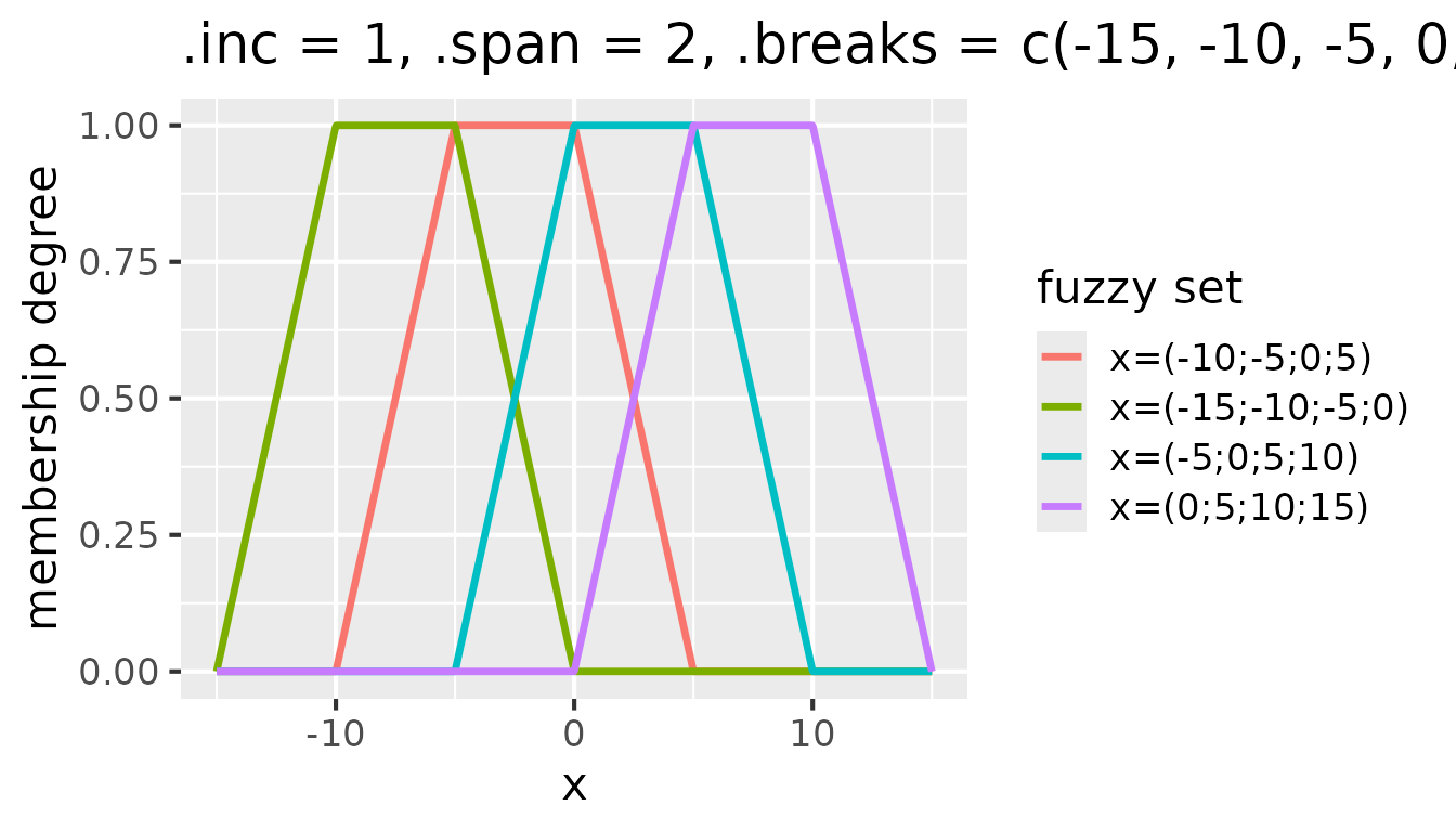
Fuzzy sets with triangular membership functions for
partition(x, .method = "triangle", .inc = 1, .span = 2, .breaks = c(-15, -10, -5, 0, 5, 10, 15))
Setting .inc to a value greater than 1 modifies the
shift of the window along the break points. For example, with
.inc = 3, the window shifts by three break points, which
effectively skips two fuzzy sets after each created fuzzy set:
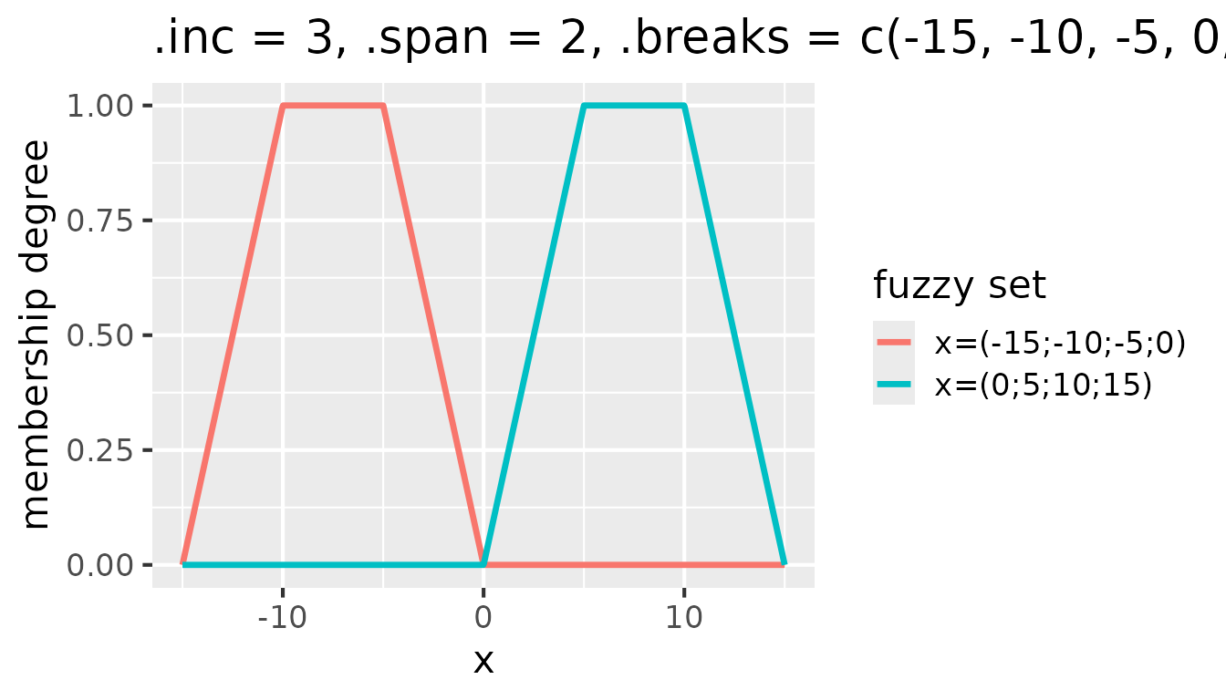
Fuzzy sets with triangular membership functions for
partition(x, .method = "triangle", .inc = 3, .span = 2, .breaks = c(-15, -10, -5, 0, 5, 10, 15))
Identifying and Removing Uninformative Columns
When preparing data for pattern discovery, it is important to
identify and potentially remove columns that provide little or no useful
information. The nuggets package provides two functions for
this purpose: is_almost_constant() and
remove_almost_constant().
Testing for Almost Constant Columns
The is_almost_constant() function checks whether a
vector contains (almost) the same value in the majority of its elements.
This is useful for detecting low-variability or degenerate
variables.
The function returns TRUE if the proportion of the most
frequent value in the vector is greater than or equal to a specified
threshold (default is 1.0, meaning completely constant).
# Completely constant vector
is_almost_constant(c(1, 1, 1, 1, 1))
#> [1] TRUE

# Variable vector
is_almost_constant(c(1, 2, 3, 4, 5))
#> [1] FALSE

# Almost constant (80% are the same value)
is_almost_constant(c(1, 1, 1, 1, 2), threshold = 0.8)
#> [1] TRUE

# Not almost constant with threshold 0.8
is_almost_constant(c(1, 1, 1, 2, 2), threshold = 0.8)
#> [1] FALSE
The function also handles NA values appropriately:
# With NA values - by default NA is treated as a regular value
is_almost_constant(c(NA, NA, NA, 1, 2), threshold = 0.5)
#> [1] TRUE

# With NA removed before computing proportions
is_almost_constant(c(NA, NA, NA, 1, 2), threshold = 0.5, na_rm = TRUE)
#> [1] TRUE
Removing Almost Constant Columns
The remove_almost_constant() function extends
is_almost_constant() to work on entire data frames. It
tests all selected columns and removes those that are almost constant
according to the specified threshold.
# Create a data frame with some constant and variable columns
d <- data.frame(
  a1 = 1:10,              # variable
  a2 = c(1:9, NA),        # variable
  b1 = "b",               # constant
  b2 = NA,                # constant (all NA)
  c1 = rep(c(TRUE, FALSE), 5),  # variable
  c2 = rep(c(TRUE, NA), 5),     # 50% TRUE, 50% NA
  d  = c(rep(TRUE, 4), rep(FALSE, 4), NA, NA)  # 40% TRUE, 40% FALSE, 20% NA
)

# Remove columns that are completely constant
remove_almost_constant(d, .threshold = 1.0, .na_rm = FALSE)
#> # A tibble: 10 × 5
#>       a1    a2 c1    c2    d
#>    <int> <int> <lgl> <lgl> <lgl>
#>  1     1     1 TRUE  TRUE  TRUE
#>  2     2     2 FALSE NA    TRUE
#>  3     3     3 TRUE  TRUE  TRUE
#>  4     4     4 FALSE NA    TRUE
#>  5     5     5 TRUE  TRUE  FALSE
#>  6     6     6 FALSE NA    FALSE
#>  7     7     7 TRUE  TRUE  FALSE
#>  8     8     8 FALSE NA    FALSE
#>  9     9     9 TRUE  TRUE  NA
#> 10    10    NA FALSE NA    NA

# Remove columns where the majority value occurs in >= 50% of rows
remove_almost_constant(d, .threshold = 0.5, .na_rm = FALSE)
#> # A tibble: 10 × 3
#>       a1    a2 d
#>    <int> <int> <lgl>
#>  1     1     1 TRUE
#>  2     2     2 TRUE
#>  3     3     3 TRUE
#>  4     4     4 TRUE
#>  5     5     5 FALSE
#>  6     6     6 FALSE
#>  7     7     7 FALSE
#>  8     8     8 FALSE
#>  9     9     9 NA
#> 10    10    NA NA

# Same as above, but removing NA before computing proportions
remove_almost_constant(d, .threshold = 0.5, .na_rm = TRUE)
#> # A tibble: 10 × 2
#>       a1    a2
#>    <int> <int>
#>  1     1     1
#>  2     2     2
#>  3     3     3
#>  4     4     4
#>  5     5     5
#>  6     6     6
#>  7     7     7
#>  8     8     8
#>  9     9     9
#> 10    10    NA
You can also restrict the check to a subset of columns using tidyselect syntax:
# Only check columns a1 through b2
remove_almost_constant(d, a1:b2, .threshold = 0.5, .na_rm = TRUE)
#> # A tibble: 10 × 5
#>       a1    a2 c1    c2    d
#>    <int> <int> <lgl> <lgl> <lgl>
#>  1     1     1 TRUE  TRUE  TRUE
#>  2     2     2 FALSE NA    TRUE
#>  3     3     3 TRUE  TRUE  TRUE
#>  4     4     4 FALSE NA    TRUE
#>  5     5     5 TRUE  TRUE  FALSE
#>  6     6     6 FALSE NA    FALSE
#>  7     7     7 TRUE  TRUE  FALSE
#>  8     8     8 FALSE NA    FALSE
#>  9     9     9 TRUE  TRUE  NA
#> 10    10    NA FALSE NA    NA
This function is particularly useful after applying
partition() to a dataset. Some of the generated predicates
may be (almost) constant and thus uninformative for pattern discovery.
Removing them can significantly speed up the subsequent mining
process.
For example:
# Prepare mtcars data with partition - use fresh copy
prepared_data <- mtcars |>
    mutate(cyl = factor(cyl, levels = c(4, 6, 8), labels = c("four", "six", "eight"))) |>
    partition(cyl, vs:gear, .method = "dummy") |>
    partition(mpg:carb, .method = "crisp", .breaks = 3)

# Check for and remove any almost constant columns
prepared_data <- remove_almost_constant(prepared_data,
                                       .threshold = 0.95,
                                       .verbose = TRUE)
Finding Tautologies in Data
After preparing your data with partition() or other
methods, it can be useful to identify tautologies—rules that are always
or almost always true in your dataset. The
dig_tautologies() function helps find such patterns, which
can then be used to filter out redundant conditions in subsequent
pattern discovery.
What are Tautologies?
A tautology in this context is a rule of the form
{a1 & a2 & ... & an} => {c} where the
antecedent (left side) almost always implies the consequent (right
side). These are rules that hold with very high confidence in your
specific dataset.
For example, in a dataset about vehicles, you might discover: -
engine_type=electric => fuel_type=electricity
(confidence ≈ 1.0) -
manual_transmission=TRUE => automatic_transmission=FALSE
(confidence = 1.0)
Such tautological rules, while true, may not provide interesting insights for further analysis. Identifying them allows you to exclude similar conditions from more complex pattern searches.
Using dig_tautologies()
The dig_tautologies() function works similarly to
dig_associations(), but is specifically optimized for
finding rules with very high confidence. It searches iteratively, using
tautologies found in earlier iterations to prune the search space in
later iterations.
Basic usage:
# Prepare fuzzy data - use fresh copy of mtcars
fuzzy_mtcars <- mtcars |>
    mutate(cyl = factor(cyl, levels = c(4, 6, 8), labels = c("four", "six", "eight"))) |>
    partition(cyl, vs:gear, .method = "dummy") |>
    partition(mpg:carb, .method = "triangle", .breaks = 3)

# Create disjoint vector
disj <- var_names(colnames(fuzzy_mtcars))

# Find tautologies with very high confidence
tautologies <- dig_tautologies(
    fuzzy_mtcars,
    antecedent = everything(),
    consequent = everything(),
    disjoint = disj,
    min_confidence = 0.95,
    min_support = 0.1,
    max_length = 3,
    t_norm = "goguen"
)

print(tautologies)
#> # A tibble: 0 × 0
The function returns a tibble in the same format as
dig_associations(), containing rules with their quality
measures (support, confidence, etc.).
Parameters
Key parameters for dig_tautologies() include:
antecedentandconsequent: Tidyselect expressions defining which columns can appear on each side of the rule.disjoint: A vector specifying mutually exclusive predicates (predicates that should not appear together in the same condition).min_confidence: The minimum confidence threshold. For tautologies, this should typically be set high (e.g., 0.9 or 0.95).min_support: The minimum support threshold. This ensures the tautology is based on a sufficient number of observations.max_length: The maximum number of predicates in the antecedent.t_norm: The t-norm to use for fuzzy conjunction ("goedel","goguen", or"lukas").
Using Tautologies to Filter Searches
Once you’ve identified tautologies, you can use them with the
excluded argument of dig() or related
functions to avoid generating similar conditions:
# Convert tautologies to excluded format
excluded_conditions <- parse_condition(tautologies$antecedent)

# Use in subsequent pattern search
results <- dig_associations(
    fuzzy_mtcars,
    antecedent = !starts_with("am"),
    consequent = starts_with("am"),
    disjoint = disj,
    excluded = excluded_conditions,  # Exclude tautological patterns
    min_support = 0.1,
    min_confidence = 0.8
)
This approach can significantly reduce computation time and help focus on more interesting patterns.
Summary
This vignette covered the essential data preparation techniques in
the nuggets package:
-
partition(): The primary function for transforming data into crisp or fuzzy predicates, with support for various partitioning methods including:- Crisp (Boolean) partitioning with configurable intervals
- Triangular and raised-cosine fuzzy sets
- Trapezoidal fuzzy sets using
.spanand.incparameters
is_almost_constant()andremove_almost_constant(): Utility functions for identifying and removing uninformative columns that have low variability.dig_tautologies(): A function for finding tautological rules in your data, which can be used to filter subsequent pattern searches.
With these tools, you can effectively prepare your data for pattern
discovery using the various dig_*() functions provided by
the nuggets package. For information on pattern discovery
itself, see the main “Getting Started” vignette and the function
documentation.